Constant Q transform
In mathematics and signal processing, the Constant Q Transform transforms a data series to the frequency domain. It is related to the Fourier Transform,[1] and very closely related to the complex Morlet wavelet transform.[2]
The transform can be thought of as a series of logarithmically spaced filters, with the k-th filter having a spectral width some multiple of the previous filter's width, i.e.

where δfk is the bandwidth of the kth filter, fmin is the centre frequency of the lowest filter, and n is the number of filters per octave.
Contents
Calculation of the Transform
The short-time Fourier Transform of x[n] for a frame shifted to sample m is calculated as follows:
![X[k,m] = \sum_{n=0}^{N-1} W[n-m] x[n] e^ { \frac{-j 2 \pi k n}{N}}](/w/images/math/1/3/7/13734a5dea80a09ff20d3fee8ec55289.png)
Given a data series, sampled at fs = 1/T, T being the sampling period of our data, for each frequency bin we can define the following:
- Filter width, δfk
- Q, the "quality factor". This is shown below to be the integer number of cycles processed at a center frequency fk. As such, this somewhat defines the time complexity of the transform.

- Window length for the k-th bin
![N[k] = \left( \frac {f_s}{\delta f_k} \right) = \left( \frac {S}{f_k} \right) Q](/w/images/math/b/7/5/b75228727c6ec86a78336ee96f156a6b.png)
- As S/fk is the number of samples processed per cycle at frequency fk, Q is the number of integer cycles processed at this center frequency.
The equivalent transform kernel can be found by using the following substitutions:
- The window length of each bin is now a function of the bin number:
![N = N[k] = Q \frac {f_s}{f_k}](/w/images/math/8/4/d/84d3abd90c4c6dd43885ec8adad30ecb.png)
- The relative power of each bin will decrease with higher frequencies, as these sum over fewer terms. To compensate for this, we normalize by N[k].
- Any windowing function will be a function of window length, and likewise a function of window number. For example, the equivalent Hamming window would be,
![W[k,n] = \alpha - \left(1 - \alpha \right) \cos \left( \frac {2 \pi n}{N[k]} \right), \alpha = 25/46 , 0 \leqslant n \leqslant N[k] - 1](/w/images/math/9/c/3/9c3e07ea9c3e951034d4681c38cd310e.png)
- Our digital frequency,
 , becomes
 ![\frac {2 \pi Q}{N[k]}](/w/images/math/b/6/7/b67969da349efdef605e5abbbc29c065.png)
After these modifications, we are left with:
![X[k] = \frac {1}{N[k]} \sum_{n=0}^{N[k]-1} W[k,n] x[n] e^{\frac{-j2 \pi Qn}{N[k]}}](/w/images/math/0/a/1/0a19a7dc16f5d4c8d422647e68dc1506.png)
Fast calculation using FFT
The direct calculation of the Constant Q transform is slow when compared against the Fast Fourier Transform (FFT). However, the FFT can itself be employed, in conjunction with the use of a kernel, to perform the equivalent calculation but much faster.[3]
Comparison with the Fourier Transform
In general, the transform is well suited to musical data, and this can be seen in some of its advantages compared to the Fast Fourier Transform. As the output of the transform is effectively amplitude/phase against log frequency, fewer frequency bins are required to cover a given range effectively, and this proves useful where frequencies span several octaves. As the range of human hearing covers approximately ten octaves from 20 Hz to around 20 kHz, this reduction in output data is significant.
The transform exhibits a reduction in frequency resolution with higher frequency bins—which is desirable for auditory applications. The transform mirrors the human auditory system, whereby at lower frequencies spectral resolution is better, whereas temporal resolution improves at higher frequencies. At the bottom of the piano scale (about 30 Hz), a difference of 1 semitone is a difference of approximately 1.5 Hz, whereas at the top of the musical scale (about 5 kHz), a difference of 1 semitone is a difference of approximately 200 Hz.[4] So for musical data the exponential frequency resolution of Constant Q is ideal.
In addition, the harmonics of musical notes form a pattern characteristic of the timbre of the instrument in this transform. Assuming the same relative strengths of each harmonic, as the fundamental frequency changes, the relative position of these harmonics remains constant. This can make identification of instruments much easier.
Relative to the Fourier Transform, implementation of this transform is more tricky. This is due to the varying number of samples used in the calculation of each frequency bin, which also affects the length of any windowing function implemented.
Also note that because the frequency scale is logarithmic, there is no true zero-frequency / DC term present, perhaps limiting possible utility of the transform.
References
- ↑ Judith C. Brown, Calculation of a constant Q spectral transform, J. Acoust. Soc. Am., 89(1):425–434, 1991.
- ↑ Continuous Wavelet Transform "When the mother wavelet can be interpreted as a windowed sinusoid (such as the Morlet wavelet), the wavelet transform can be interpreted as a constant-Q Fourier transform. Before the theory of wavelets, constant-Q Fourier transforms (such as obtained from a classic third-octave filter bank) were not easy to invert, because the basis signals were not orthogonal."
- ↑ Judith C. Brown and Miller S. Puckette, An efficient algorithm for the calculation of a constant Q transform, J. Acoust. Soc. Am., 92(5):2698–2701, 1992.
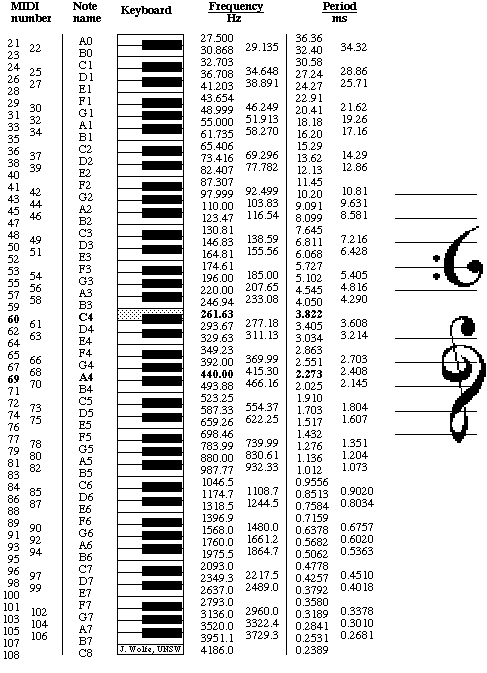
- ↑ http://newt.phys.unsw.edu.au/jw/graphics/notes.GIF